Distributions

1. Last week I did a thread on the law of large numbers (LLN): https://twitter.com/rahuldave/status/1425883481821704192 or https://stories.univ.ai/lawoflargenumbers/. The essence was that the mean of N random variables drawn from a distribution converge to the mean µ of the distribution as N becomes infinite.

2. Remember that a random variable is one that can take multiple values, each with some probability. So if X represents the flip of a coin, it will take values Heads and Tails with some probability. We'll assign Heads the value 1 and Tails the value 0.

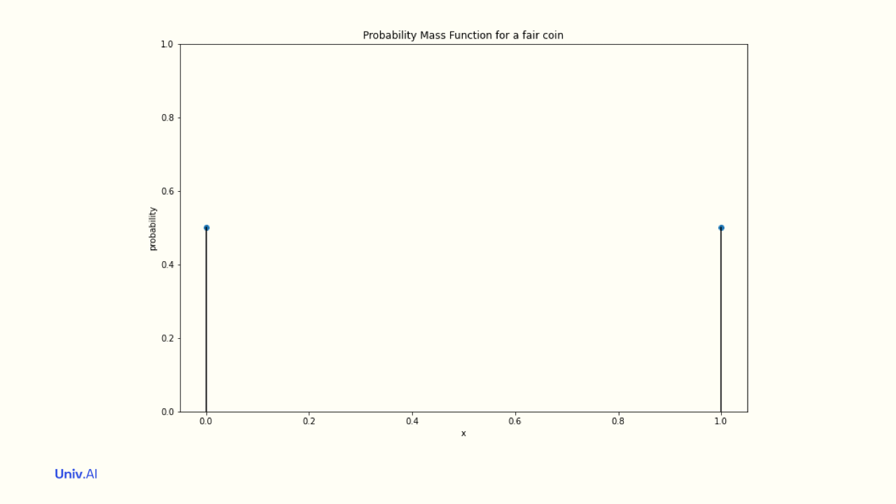
3. The probabilities attached to the values a random variable takes is called a distribution, or probability mass function (pmf). For a single fair coin, the "Bernoulli" Distribution attaches probabilities 0.5 to value 1 and 0.5 to value 0. These probabilities must add to 1.

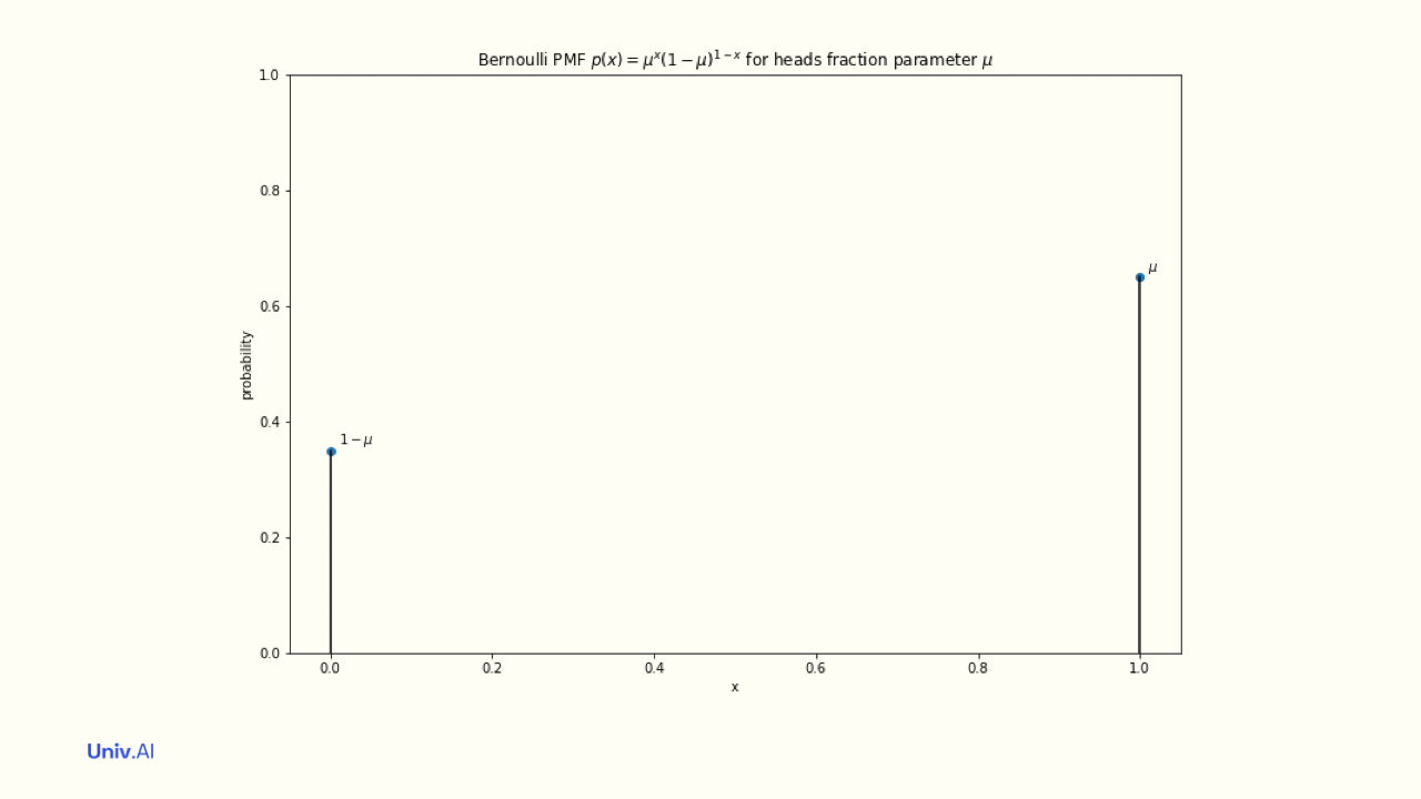
4. The Bernoulli Distribution is a Discrete Distribution for a single coin toss with probability parameter µ. Its pmf associates a probability of µ with value 1. The LLN says that if you toss the coin N times, the fraction of heads converges to µ as N becomes infinite.

5. Another example of a discrete distribution is the Binomial Distribution. It answers the question: what is the probability of getting k heads in N coin tosses, given the intrinsic probability µ?

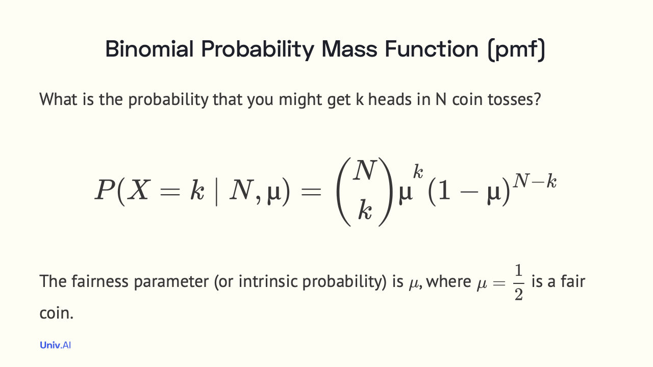
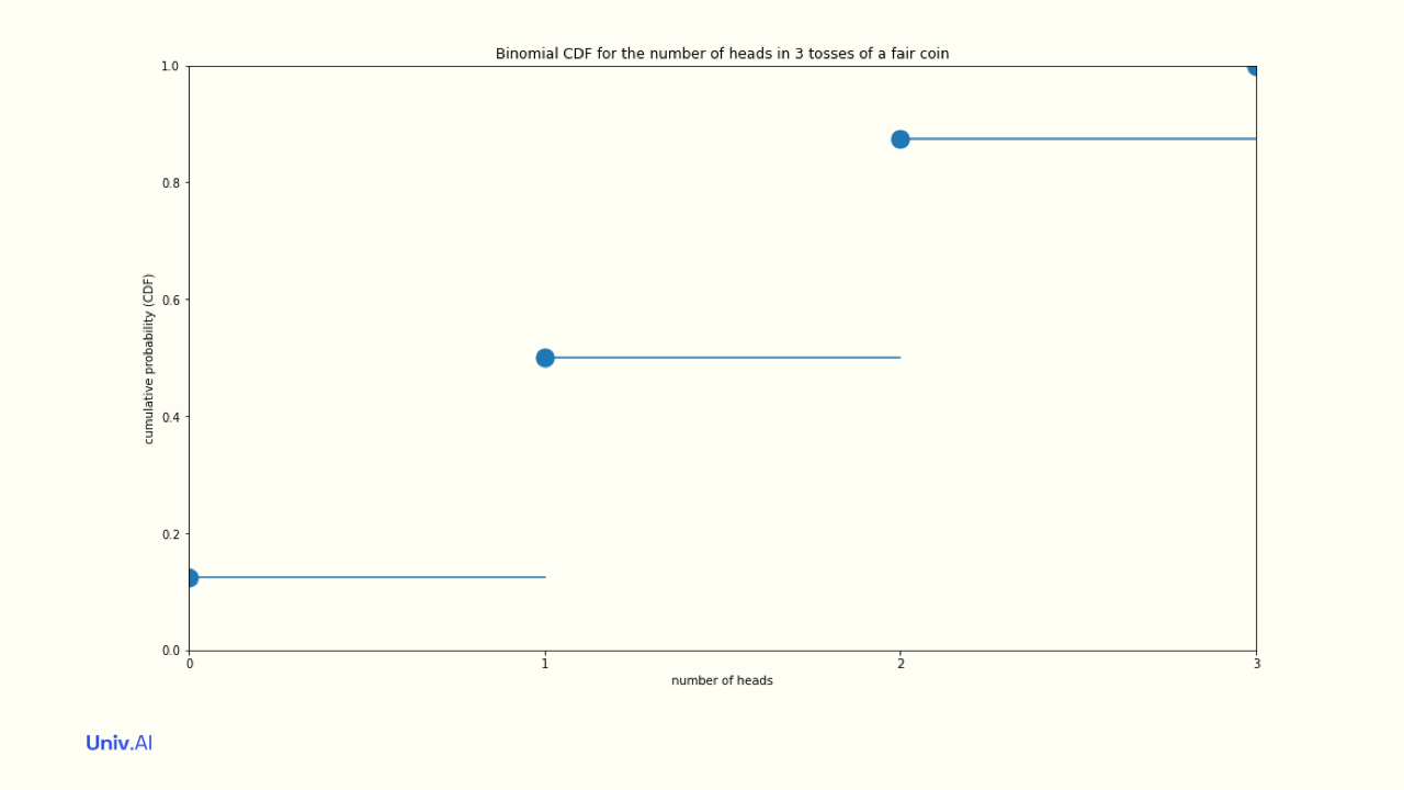
6. For example, what is the intrinsic probability of getting 2 out of 3 heads for a fair coin? The probability is (1/2)^2 for heads times (1/2) for tails (1/8), added up for the number of ways this can happen, which, as can be seen in the image, is 3. So 1/8 + 1/8 + 1/8 = 3/8.

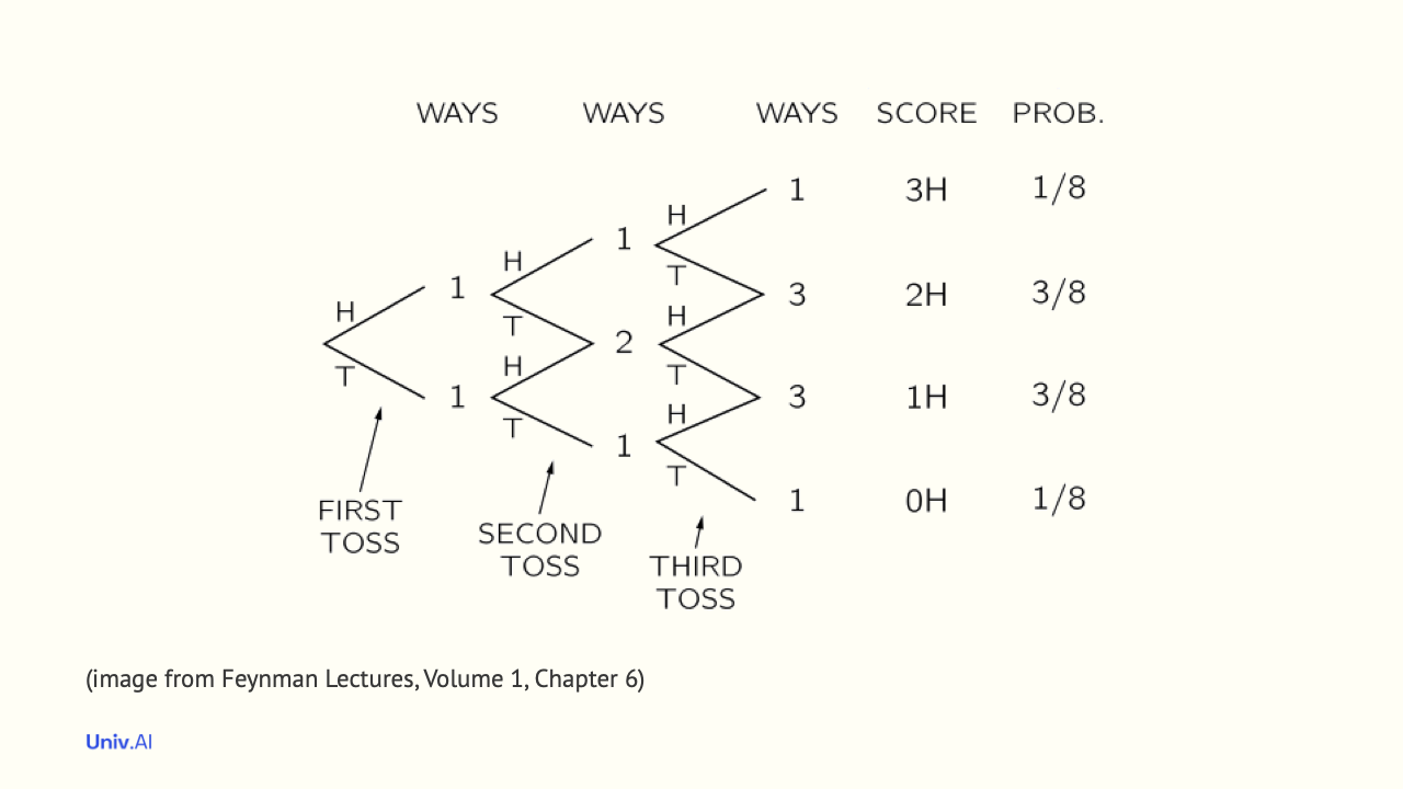
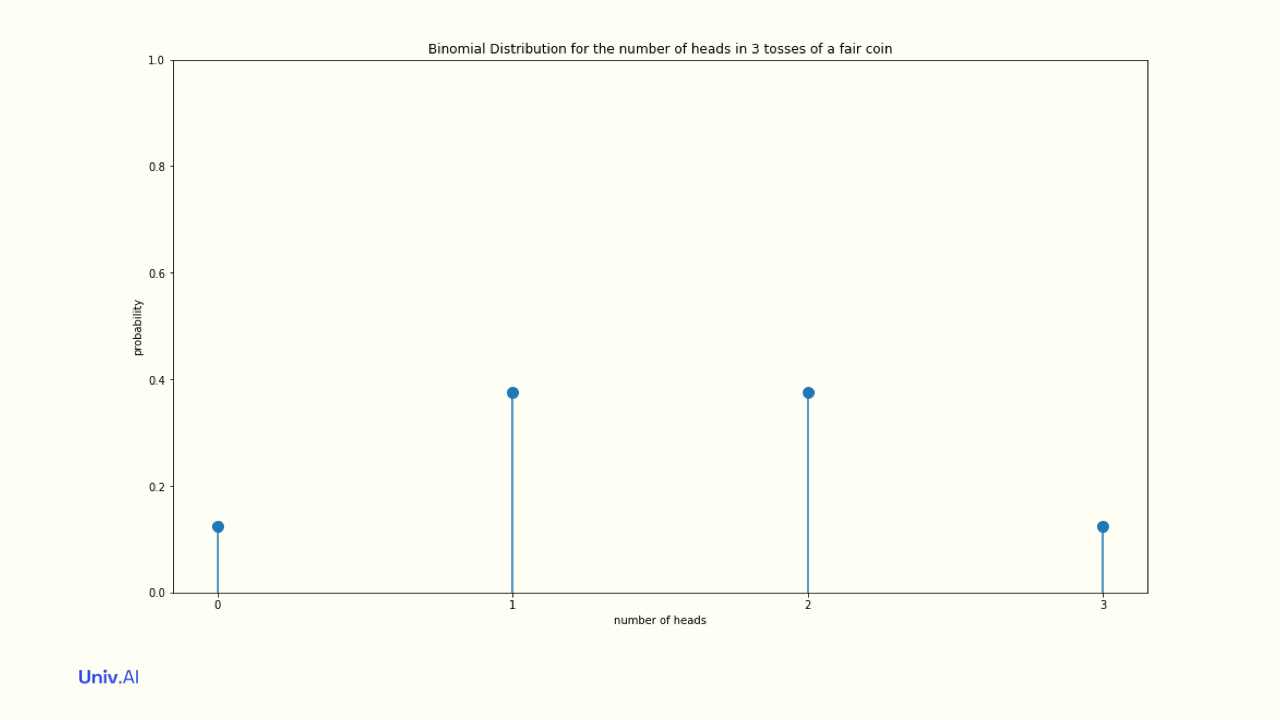
7. The probabilities of all the options in the pmf, that is k=0, k=1, k=2, and k=3 heads must add to 1. And if you repeated the experiment of tossing 3 coins N times, the LLN tells us that as N becomes infinite, the fraction of times you get 2 heads converges to 3/8.

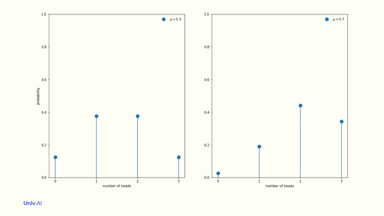
8. What happens if you change the coin bias or probability parameter to µ=0.7? Then heads is more likely as compared to the fair coin case. So the pmf shifts to higher probabilities for larger k.

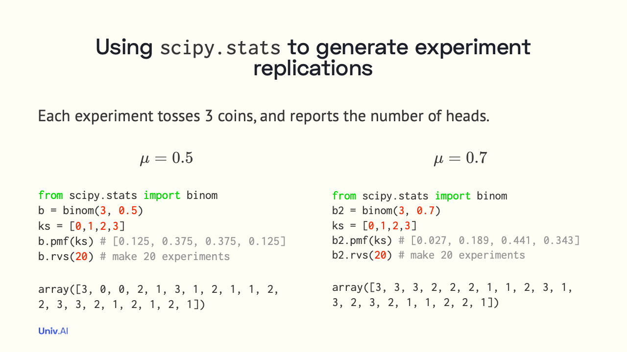
9. pmf's tell us probabilities for our random variable. But, probability distributions are most useful when you use them to generate new data. For example, you might do simulations of 100 experiments of 3 coin tosses and see how many heads you get in each.

10. What about a continuous random variable X, like the heights of people? In this case one defines a probability density function (pdf) p(x), the probability density that X=x (say 6 feet).

11. The area of an infinitesimally thin (width dx) rectangular sliver at X=x (yellow) with height the pdf p(x) is p(x)dx . This represents the probability that the random variable X has its value between x and x+dx. The sum of these areas in the range of X must be 1!

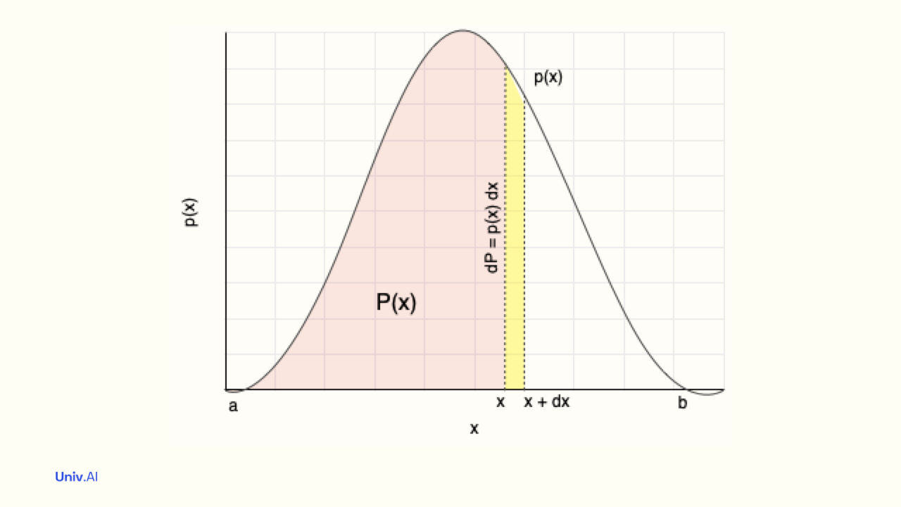
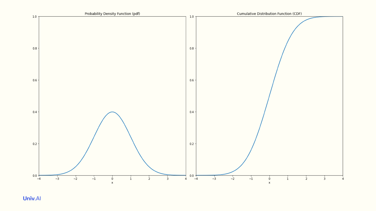
12. The area upto X=x (pink) is called the Cumulative Distribution Function (CDF) P(x). It is the probability that the random variable X has value less than or equal to x. P(x) must always between 0 and 1. For calculus lovers, the integral of the pdf upto x is the CDF.

13. A famous continuous distribution is the Gaussian Distribution, arising in many real-life situations such as human weights, elections, etc. The pdf is much lower in values than the CDF, since the area under the pdf (NOT the sum of its values) must be 1.

14. The CDF can be defined for discrete probability distributions as well. There we simply add the probability upto and including x, rather than having to compute the area.

15. Distributions are everywhere. For example, predicting elections and doing linear regression involve Gaussian Distributions. We'll tackle these in future tweet threads. Follow me on twitter at @rahuldave and keep an eye on https://stories.univ.ai for more!

16. Permalink to thread here: https://stories.univ.ai/distributions/! If you'd like to learn Data Science and AI, you might want to check out our programs at https://univ.ai/programs/, and the thread https://twitter.com/rahuldave/status/1424793241019428864 (discounts inside).